Cost-Sensitive Customer Churn Prediction
Table of Contents

Predicting customer churn is not just about identifying who is likely to leave; it’s about understanding the financial implications behind each customer’s departure. In addition, one of the complexities in churn prediction is dealing with imbalanced datasets, where the number of non-churning customers vastly outnumbers the churning ones.
Today, I’ll build a cost-sensitive customer churn prediction model using machine learning. I’ll delve into data exploration, feature engineering, model training, and evaluation with the goal to minimize financial losses associated with customer churn. At the same time, I’ll analyze the performance of a classification model during an imbalance dataset scenario.
Introduction #
Customer churn is a critical metric for businesses, especially in industries like telecommunications, banking, and subscription-based services. Churn prediction models help identify customers who are likely to discontinue using a company’s products or services. By proactively addressing churn, companies can implement targeted retention strategies, thereby saving significant revenue.
Traditional churn prediction models often focus solely on accuracy, neglecting the financial ramifications of different types of prediction errors. For instance, the cost of incorrectly predicting that a loyal customer will churn (false positive) is different from failing to identify a churning customer (false negative). To address this, I adopt a cost-sensitive approach that incorporates the business costs associated with each type of error directly into the model.
In this post, I’ll build a churn prediction model that considers these costs. Plus, I’ll address the issue of class imbalance, where most data points are for non-churn customers. Imbalance like this can make the model overlook actual churners, which isn’t helpful for a business looking to keep customers around.
Business Scenario #
Before diving into the data and code, it’s essential to frame our problem in a real-world business context. Our goal is not just to predict churn but to minimize the financial impact of churn on the business.
The Cost Matrix #
Define a cost matrix that quantifies the financial consequences of different prediction outcomes:
| Predicted Stay (0) | Predicted Churn (1) | |
|---|---|---|
| Actual Stay (0) | $0 | -$200 |
| Actual Churn (1) | -$750 | $550 |
- True Negative (TN): Correctly predicting a customer will stay. Cost: $0.
- False Positive (FP): Predicting a customer will churn when they won’t. Cost: -$200 (cost of unnecessary retention efforts).
- False Negative (FN): Failing to predict a customer will churn. Cost: -$750 (loss due to customer leaving).
- True Positive (TP): Correctly predicting a customer will churn and taking action. Gain: $550 (benefit from retaining the customer).
Note: Negative costs represent expenses, while positive costs represent gains.
By integrating this cost matrix into our model, I ensure that our predictions align with business objectives, focusing on maximizing profit rather than just statistical accuracy.
Understanding the Class Imbalance Problem #
Class imbalance occurs when one class in a classification problem is represented much more than other classes. In churn prediction, typically, most customers do not churn, leading to an imbalanced dataset. This imbalance can bias models towards the majority class, causing poor performance in predicting the minority class.
There is ongoing debate in the data science community about the best approach to handle class imbalance:
- Resampling Techniques: Such as oversampling the minority class or undersampling the majority class.
- Class Weighting: Assigning higher weights to the minority class during model training.
- Algorithmic Adjustments: Using algorithms that are robust to class imbalance.
- Leave Data As-Is: Some argue that altering the dataset may distort the true distribution, and models should learn from the original data.
In this project, I focus on applying class weighting and compare it with models trained on the original imbalanced data.
Dataset Overview #
The dataset used in this project is sourced from Kaggle’s Bank Customer Churn Dataset by Radheshyam Kollipara.
The dataset includes the following features:
- RowNumber: Represents the row number.
- CustomerId: Unique identifier for each customer.
- Surname: The last name of the customer.
- CreditScore: Credit score of the customer.
- Geography: Country of residence.
- Gender: Customer’s gender.
- Age: Customer’s age.
- Tenure: Number of years the customer has been with the bank.
- Balance: Customer’s account balance.
- NumOfProducts: Number of bank products the customer is using.
- HasCrCard: Indicates if the customer has a credit card (1) or not (0).
- IsActiveMember: Indicates if the customer is an active member (1) or not (0).
- EstimatedSalary: Estimated annual income of the customer.
- Exited: Target variable showing whether the customer has churned (1) or stayed (0).
- Complain: Indicates if the customer has filed a complaint (1) or not (0).
- Satisfaction Score: Customer satisfaction score (1-5).
- Card Type: Type of card held by the customer (e.g., Silver, Gold).
- Points Earned: Loyalty points accumulated by the customer.
Dataset preview:
dataset.sample(5)
| RowNumber | CustomerId | Surname | CreditScore | Geography | Gender | Age | Tenure | Balance | NumOfProducts | HasCrCard | IsActiveMember | EstimatedSalary | Exited | Complain | Satisfaction Score | Card Type | Point Earned | |
|---|---|---|---|---|---|---|---|---|---|---|---|---|---|---|---|---|---|---|
| 2503 | 2504 | 15583364 | McGregor | 476 | France | Female | 32 | 6 | 111871.93 | 1 | 0 | 0 | 112132.86 | 0 | 0 | 3 | GOLD | 988 |
| 1362 | 1363 | 15683841 | Hamilton | 555 | Germany | Male | 41 | 10 | 113270.20 | 2 | 1 | 1 | 185387.14 | 0 | 0 | 1 | SILVER | 398 |
| 842 | 843 | 15599433 | Fanucci | 660 | Germany | Male | 35 | 8 | 58641.43 | 1 | 0 | 1 | 198674.08 | 0 | 0 | 5 | PLATINUM | 815 |
| 7919 | 7920 | 15634564 | Aksyonov | 593 | Spain | Male | 31 | 8 | 112713.34 | 1 | 1 | 1 | 176868.89 | 0 | 0 | 2 | GOLD | 710 |
| 3512 | 3513 | 15657779 | Boylan | 806 | Spain | Male | 18 | 3 | 0.00 | 2 | 1 | 1 | 86994.54 | 0 | 0 | 2 | GOLD | 768 |
Exploratory Data Analysis (EDA) #
Data Cleaning #
First, let’s check for missing values:
dataset.isnull().sum()
Result:
CustomerId            0
CreditScore           0
Geography             0
Gender                0
Age                   0
Tenure                0
Balance               0
NumOfProducts         0
HasCrCard             0
IsActiveMember        0
EstimatedSalary       0
Exited                0
Complain              0
Satisfaction Score    0
Card Type             0
Point Earned          0
dtype: int64
All columns have zero missing values.
Next, let’s drop irrelevant columns that won’t contribute to our project’s objective:
data.drop(columns=['RowNumber', 'CustomerId', 'Surname'], inplace=True)
Statistical Summary #
Generate a statistical summary to understand the distribution of numerical features:
data.describe()
| CustomerId | CreditScore | Age | Tenure | Balance | NumOfProducts | HasCrCard | IsActiveMember | EstimatedSalary | Exited | Complain | Satisfaction Score | Point Earned | |
|---|---|---|---|---|---|---|---|---|---|---|---|---|---|
| count | 10000 | 10000 | 10000 | 10000 | 10000 | 10000 | 10000 | 10000 | 10000 | 10000 | 10000 | 10000 | 10000 |
| mean | 1.56909e+07 | 650.529 | 38.9218 | 5.0128 | 76485.9 | 1.5302 | 0.7055 | 0.5151 | 100090 | 0.2038 | 0.2044 | 3.0138 | 606.515 |
| std | 71936.2 | 96.6533 | 10.4878 | 2.89217 | 62397.4 | 0.581654 | 0.45584 | 0.499797 | 57510.5 | 0.4028 | 0.4033 | 1.40592 | 225.925 |
| min | 1.55657e+07 | 350 | 18 | 0 | 0 | 1 | 0 | 0 | 11.58 | 0 | 0 | 1 | 119 |
| 25% | 1.56285e+07 | 584 | 32 | 3 | 0 | 1 | 0 | 0 | 51002.1 | 0 | 0 | 2 | 410 |
| 50% | 1.56907e+07 | 652 | 37 | 5 | 97198.5 | 1 | 1 | 1 | 100194 | 0 | 0 | 3 | 605 |
| 75% | 1.57532e+07 | 718 | 44 | 7 | 127644 | 2 | 1 | 1 | 149388 | 0 | 0 | 4 | 801 |
| max | 1.58157e+07 | 850 | 92 | 10 | 250898 | 4 | 1 | 1 | 199992 | 1 | 1 | 5 | 1000 |
Insights:
- Age: Mean age is around 39 years, with a standard deviation of 10.5 years.
- Balance: Average balance is \( \$76,486 \), but the standard deviation is high $62,397, indicating significant variability.
- Exited: Approximately 20% of customers have churned, showing class imbalance.
Handling Class Imbalance #
Class imbalance can bias the model towards the majority class (non-churned customers). I’ll address this issue during model training using techniques like class weighting and threshold adjustment.
Feature Exploration and Engineering #
Understanding relationships between features and the target variable is crucial.
Correlation Analysis #
Compute the correlation matrix to identify linear relationships:

Key Findings:
- Age has a weak positive correlation with Exited (0.29), suggesting older customers are more likely to churn.
- Complain has a strong positive correlation with Exited (0.99). This may indicate the existance of a complain solely in churned customers.
Further analysis indicates that the strong correlation between complaints and churn is due to the fact that almost every customer who churns had filed a complaint before leaving. In contrast, customers who did not churn rarely filed complaints. This suggests that complaints are a strong indicator of dissatisfaction, which often leads to churn. This feature might lead to data leakage. I’ll consider dropping it.
complain = dataset.groupby(['Complain','Exited']).size().reset_index(name='Count')
total = complain['Count'].sum()
complain['Proportion'] = (complain['Count'] / total )
| Complain | Exited | Count | Proportion |
|---|---|---|---|
| 0 | 0 | 7952 | 0.7952 |
| 0 | 1 | 4 | 0.0004 |
| 1 | 0 | 10 | 0.001 |
| 1 | 1 | 2034 | 0.2034 |
Visualizing Key Features #
Age Distribution #
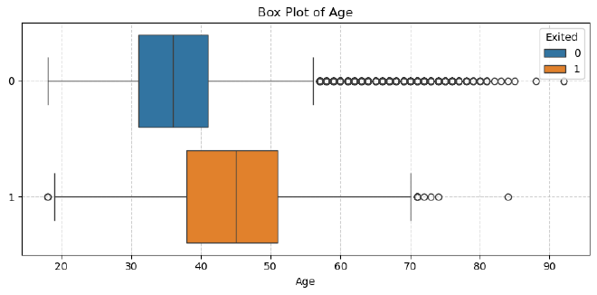
Observation:
- Churned customers tend to be older.
Balance Distribution #
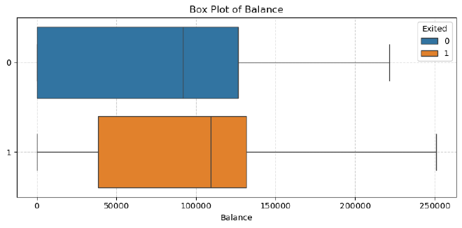
Observation:
- Churned customers generally have higher account balances.
Number of Products #
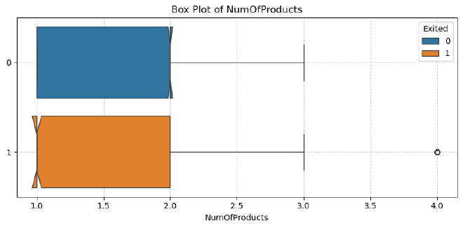
Observation:
- Customers with one product are more likely to churn than those with multiple products.
Tenure #
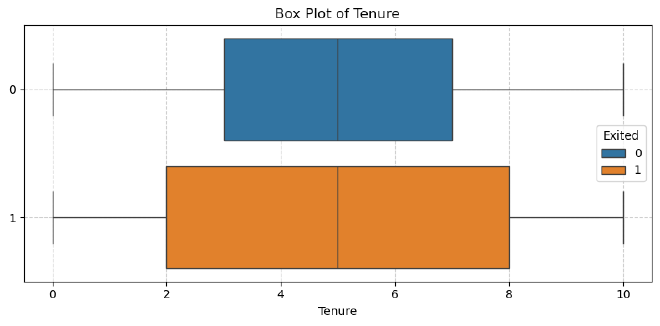
Observation:
- Tenure distribution is similar for both churned and non-churned customers, with both groups having a median tenure of 5 years.
- Churned customers display more variability in tenure, indicating they may leave at different stages in their bank relationship.
Estimated Salary #
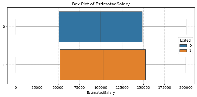
Observation:
- Churned and non-churned customers have similar median balances around 100,000.
- Both groups show a similar spread in balances with no outliers.
Satisfaction Score #
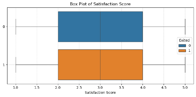
Observation:
- Both churned and non-churned customers have the same distribution, with a median of 3 and identical interquartile ranges.
- The lower and upper fences are also identical, with no outliers for either group.
Geography #
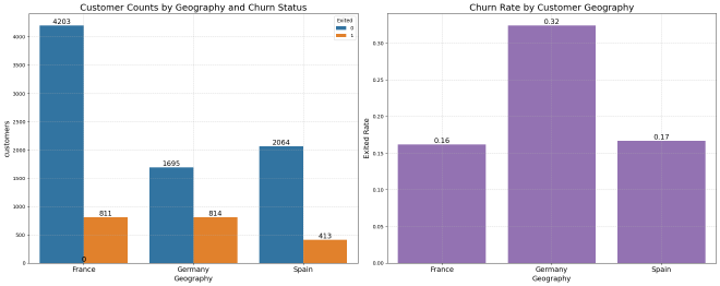
Observation:
- France: Has the largest customer base, with a churn rate of 16.2%.
- Germany: Shows a significantly higher churn rate at 32.4%, suggesting that German customers are more likely to churn.
- Spain: Has a churn rate similar to France at 16.7%.
These differences indicate that geography might influence churn, with German customers showing a higher likelihood of leaving compared to those from France and Spain.
Satisfaction Score #
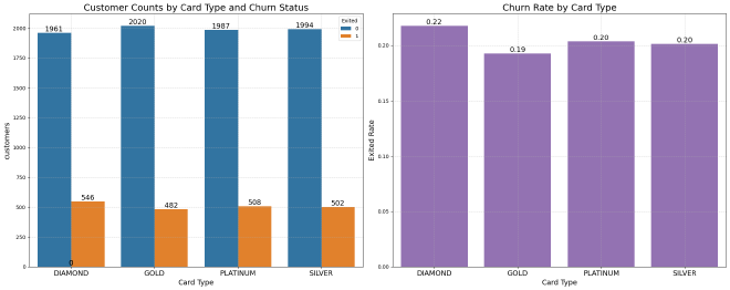
Observation:
- Diamond Card Holders: Have the highest churn rate at 21.8%.
- Gold Card Holders: Show the lowest churn rate at 19.3%.
- Platinum and Silver Card Holders: Have similar churn rates, around 20.3% and 20.1%, respectively.
These results suggest that Diamond card holders may be more likely to churn, while Gold card holders are slightly more likely to stay. However, the differences in churn rates across card types are relatively small.
Feature Extraction #
Dropping Potentially Problematic Features #
I consider dropping the Complain feature due to its near-perfect correlation with Exited, which could cause data leakage:
data.drop(columns=['CustomerId','Complain'], inplace=True)
Data Preprocessing #
Train-Test Split #
Split the data into training, validation, and test sets. This is done before the feature scalling to avoid data leakage.
from sklearn.model_selection import train_test_split

X = dataset.drop(columns='Exited')
y = dataset['Exited']

# Initial split to separate out the hold-out set
X_train_val, X_test, y_train_val, y_test = train_test_split(
    X, y, test_size=0.2, random_state=42, stratify=y)

# Split the remaining data into training and validation sets
X_train, X_val, y_train, y_val = train_test_split(
    X_train_val, y_train_val, test_size=0.25, random_state=42, stratify=y_train_val)
Based on these splits, the final distribution is:
| Dataset | Total Count | Percentage of Total Data |
|---|---|---|
| Training | 6,000 | 60% |
| Validate | 2,000 | 20% |
| Testing | 2,000 | 20% |
Column Transformer #
from sklearn.compose import ColumnTransformer
from sklearn.preprocessing import OneHotEncoder, StandardScaler

num_cols = ['CreditScore', 'Age', 'Tenure', 'Balance', 'NumOfProducts', 'EstimatedSalary', 'Satisfaction Score','Point Earned']
cat_cols = ['Geography', 'Card Type', 'Gender']
bin_cols = ['HasCrCard','IsActiveMember']

preprocessor = ColumnTransformer(
    transformers=[
        # One-hot encoding for categorical variables
        ('one_hot_encoder', OneHotEncoder(drop='first', sparse_output=False), cat_cols),
        # Standard scaling to numerical features
        ('standard_scaler', StandardScaler(), num_cols),
    ],
    # Passthrough binary features
    remainder='passthrough'
)

preprocessor.fit(X_train)

X_train = preprocessor.transform(X_train)
X_val = preprocessor.transform(X_val)
X_test = preprocessor.transform(X_test)

feature_names = list(preprocessor.named_transformers_['one_hot_encoder'] \
                            .get_feature_names_out(input_features=cat_cols))
feature_names = feature_names + num_cols + bin_cols
Defining the Cost Function #
We define a custom cost function to evaluate our models based on the business cost matrix:
from sklearn.metrics import confusion_matrix, make_scorer

def cost_function(y_true, y_pred, neg_label=0, pos_label=1):
    cm = confusion_matrix(y_true, y_pred, labels=[neg_label, pos_label])

    cost_matrix = np.array([
        [0, -200],  # [TN cost, FP cost]
        [-750, 550] # [FN cost, TP gain]
    ])

    total_gain = np.sum(cm * cost_matrix)
    return total_gain

cost_scorer = make_scorer(cost_function, greater_is_better=True, neg_label=0, pos_label=1)
This function calculates the total profit (or loss) for a set of predictions, considering the costs associated with each type of prediction outcome.
Model Training #
I’ll train three different models:
- Logistic Regression
- Random Forest Classifier
- XGBoost Classifier
Cross-Validation #
Use stratified k-fold cross-validation to ensure that each fold has a similar class distribution:
from sklearn.model_selection import cross_val_score, StratifiedKFold

skf = StratifiedKFold(n_splits=5, shuffle=True, random_state=42)
Baseline Models #
Start by training baseline models without handling class imbalance.
Logistic Regression #
from sklearn.linear_model import LogisticRegression

lr_base = LogisticRegression(random_state=42)
lr_base.fit(X_train, y_train)
Random Forest #
from sklearn.ensemble import RandomForestClassifier

rf_base = RandomForestClassifier(random_state=42)
rf_base.fit(X_train, y_train)
XGBoost #
from xgboost import XGBClassifier

#The fraction of positive instances in the y_train_val dataset
pos_frac = y_train_val.mean()

xgb_base = XGBClassifier(random_state=42, base_score=pos_frac)
xgb_base.fit(X_train, y_train)
Weighted Models #
Applied class weighting to address class imbalance.
Logistic Regression with Class Weights #
lr_balanced = LogisticRegression(random_state=42, class_weight='balanced')
lr_balanced.fit(X_train, y_train)
Random Forest with Class Weights #
rf_balanced = RandomForestClassifier(random_state=42, class_weight='balanced')
rf_balanced.fit(X_train, y_train)
XGBoost with Scale Pos Weight #
Calculate scale_pos_weight as the ratio of negative to positive classes.
from collections import Counter

counter = Counter(y_train)
neg_class = counter[0]
pos_class = counter[1]
scale_pos_weight = neg_class / pos_class

xgb_balanced = XGBClassifier(random_state=42, scale_pos_weight=scale_pos_weight, base_score=pos_frac)
xgb_balanced.fit(X_train, y_train)
Model Evaluation on Validation Data #
Evaluation Metrics #
Evaluate models using several metrics:
- Accuracy: Overall correctness.
- Precision: Correct positive predictions over total positive predictions.
- Recall: Correct positive predictions over actual positives.
- F1-Score: Harmonic mean of precision and recall.
- ROC-AUC: Area under the Receiver Operating Characteristic curve.
- MCC: Delivers a balanced assessment by considering all elements of the confusion matrix.
- Brier Score: Assesses the accuracy of probabilistic predictions by measuring the mean squared difference between predicted probabilities and actual outcomes.
| Model Name | Accuracy | Precision | Recall | F1 Score | ROC AUC | MCC |
|---|---|---|---|---|---|---|
| LR Base | 0.8040 | 0.5564 | 0.1818 | 0.2741 | 0.7719 | 0.2339 |
| LR Balanced | 0.7045 | 0.3808 | 0.7224 | 0.4987 | 0.7743 | 0.3492 |
| RF Base | 0.8610 | 0.7452 | 0.4816 | 0.5851 | 0.8418 | 0.5236 |
| RF Balanced | 0.8575 | 0.7480 | 0.4521 | 0.5636 | 0.8500 | 0.5065 |
| XGB Base | 0.8535 | 0.6696 | 0.5528 | 0.6057 | 0.8362 | 0.5203 |
| XGB Balanced | 0.8270 | 0.5695 | 0.6143 | 0.5910 | 0.8364 | 0.4821 |
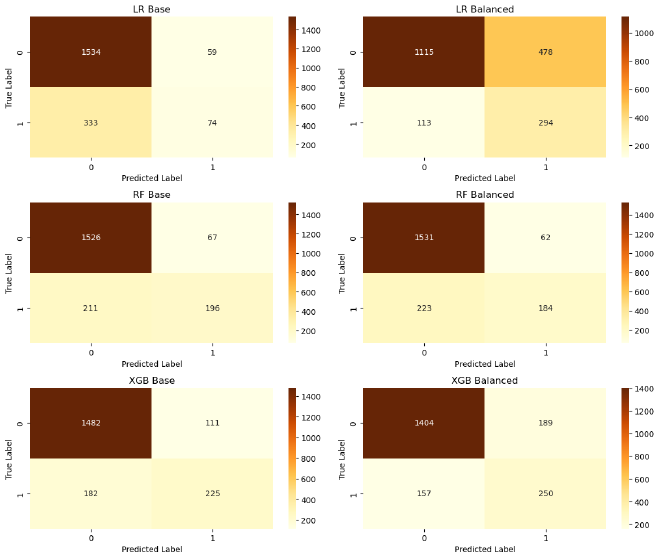
Observation:
- RF stands out with the highest MCC and ROC AUC, indicating robust performance across multiple metrics.
- While RF Balanced has the higher ROC AUC, RF Base achieves the highest MCC.
- In terms of the F1 score, XGB achieves the best results.
Cross Validated ROC AUC Scores #
| Model | ROC AUC |
|---|---|
| RF Balanced | 0.8273 |
| RF Base | 0.8256 |
| XGB Base | 0.8143 |
| XGB Balanced | 0.8075 |
| LR Balanced | 0.7659 |
| LR Base | 0.7641 |
Calibration and Feature Importance #
Calibration Plot #
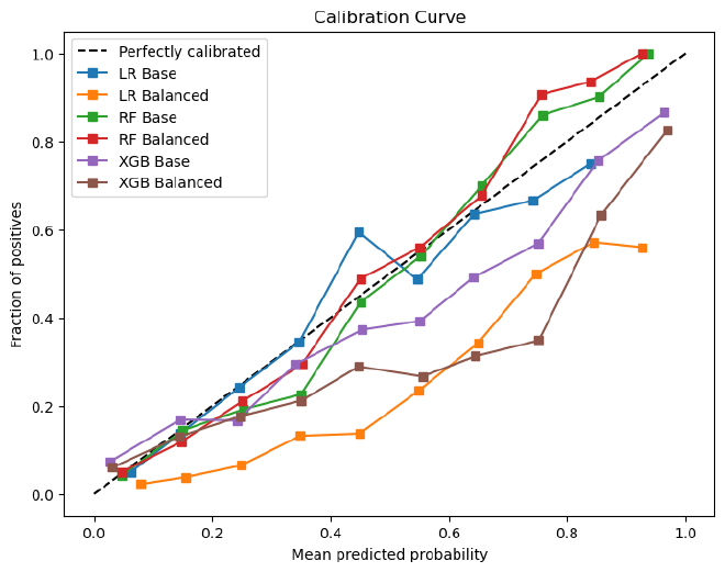
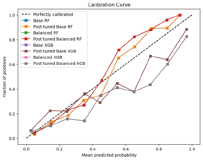
Calibration plots help assess how well predicted probabilities reflect actual probabilities.
Brier Scores (lower is better) #
| Model | Brier Score |
|---|---|
| RF Balanced | 0.1068 |
| RF Base | 0.1082 |
| XGB Base | 0.1111 |
| XGB Balanced | 0.1263 |
| LR Base | 0.1350 |
| LR Balanced | 0.1966 |
Observation:
- Balanced Random Forest has the best Brier score, making it the most accurate model for probability predictions.
- Balancing improves Random Forest slightly, but worsens performance for Logistic Regression and slightly for XGBoost.
Feature Importance #
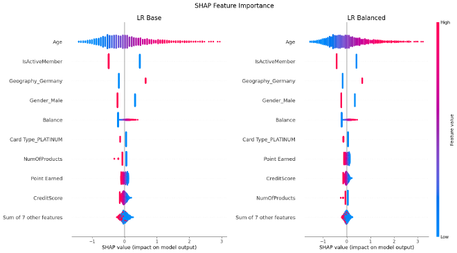
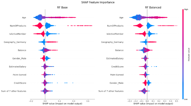
To determine the most important features, I use SHAP (SHapley Additive exPlanations) which helps to undestand how much each feature contributes to a model’s predictions.
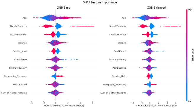
Observation:
- Age, NumOfProducts, and IsActiveMember are consistently the most important features in RF and XGB models, indicating that age, number of products and active membership status significantly influence churn.
- Balancing the dataset has little effect on feature importance for each model.
Tuning the Decision Threshold #
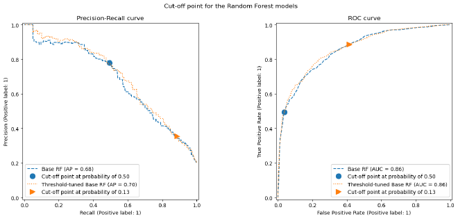
By default, models classify samples as positive if the predicted probability is ≥ 0.5. However, this threshold might not be optimal for our cost-sensitive scenario.
Threshold Tuning Process #
Search for a threshold that maximizes our custom cost function with TunedThresholdClassifierCV from scikit-learn.
from sklearn.model_selection import TunedThresholdClassifierCV

tuned_model = TunedThresholdClassifierCV(
    model,
    scoring=cost_scorer, #Custom Business Scoring
    store_cv_results=True,
)

tuned_model.fit(X_train, y_train)
Results After Threshold Tuning #
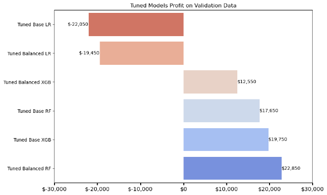
Observation:
- The Post-tuned Balanced RF model yields the highest profit at $22,850, making it the top-performing model.
- Both tuned Logistic Regression models result in negative profits.
Final Evaluation on Hold-Out Data #
Test the models on a hold-out dataset to evaluate its final performance. Due to poor performance, Logistic Regression was excluded from these evaluations.
Model Profitability #
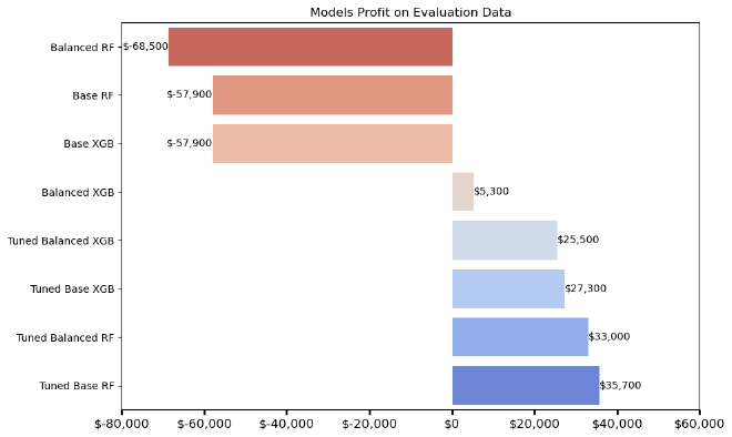
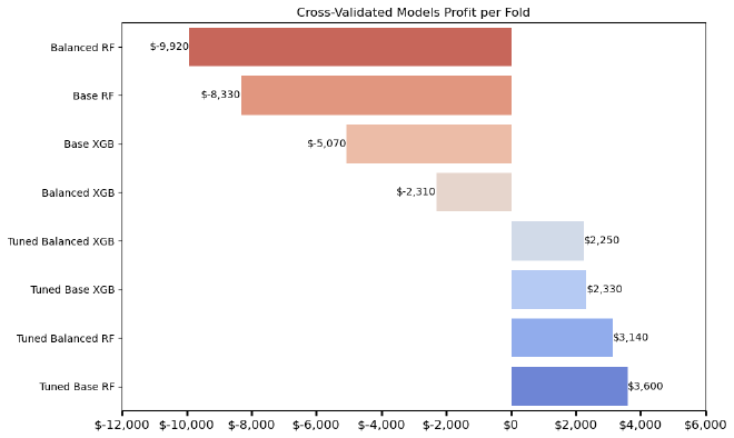
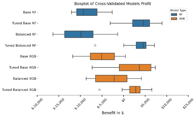
Observation:
- With the exception of Balanced XGB, the threshold-tuned models outperform all non-tuned models in terms of profit on unseen data.
- The most profitable model is the threshold-tuned Random Forest baseline.
Model Overall #
| Model Name | Accuracy | Precision | Recall | F1 Score | ROC AUC | MCC |
|---|---|---|---|---|---|---|
| Base RF | 0.8690 | 0.7897 | 0.4877 | 0.6030 | 0.8578 | 0.5518 |
| Post-tuned Base RF | 0.7125 | 0.4016 | 0.8358 | 0.5426 | 0.8578 | 0.4212 |
| Balanced RF | 0.8700 | 0.8217 | 0.4632 | 0.5925 | 0.8632 | 0.5526 |
| Post-tuned Balanced RF | 0.6480 | 0.3549 | 0.8873 | 0.5070 | 0.8632 | 0.3820 |
| Base XGB | 0.8470 | 0.6635 | 0.5074 | 0.5750 | 0.8403 | 0.4902 |
| Post-tuned Base XGB | 0.6585 | 0.3598 | 0.8652 | 0.5083 | 0.8403 | 0.3794 |
| Balanced XGB | 0.8400 | 0.5987 | 0.6544 | 0.6253 | 0.8439 | 0.5247 |
| Post-tuned Balanced XGB | 0.6980 | 0.3874 | 0.8260 | 0.5274 | 0.8439 | 0.3992 |
Best Model #
Post-tuned Random Forest #
| Model Name | Accuracy | Precision | Recall | F1 Score | ROC AUC | MCC |
|---|---|---|---|---|---|---|
| Post-tuned Base RF | 0.7125 | 0.4016 | 0.8358 | 0.5426 | 0.8578 | 0.4212 |
Conclusion #
Predicting customer churn is not just about identifying who is likely to leave, but also about understanding the financial impact of losing a customer. By adopting a cost-sensitive approach, this project aimed to align predictive modeling with business objectives, ensuring that retention strategies maximize financial gains.
The analysis demonstrated that handling class imbalance is crucial for effective churn prediction. While traditional models tend to favor the majority class, applying techniques like class weighting improved recall, allowing the model to better capture customers at risk of churning.
Among the models tested, the Post-Tuned Balanced Random Forest emerged as the most profitable option. By fine-tuning decision thresholds, this model optimized the balance between correctly identifying churners and minimizing false positives, ultimately leading to the highest financial gains on unseen data.
Moreover, feature importance analysis revealed that Age, Number of Products, and Active Membership were key drivers of churn. Understanding these factors allows businesses to develop targeted interventions to retain customers effectively.
Key Takeaways #
-
Cost-Sensitive Approach Enhances Business Alignment
Incorporating a cost matrix into the model evaluation ensured that predictions were aligned with financial outcomes rather than pure statistical accuracy. This approach helped balance profit maximization while mitigating unnecessary costs. -
Class Imbalance Affects Model Performance
The dataset exhibited a significant class imbalance, which was addressed using class weighting and cost-sensitive learning. Balanced models performed better in terms of recall, ensuring that more churn cases were correctly identified. -
Post-Tuned Random Forest Model Performed Best
After threshold tuning, the Post-tuned Balanced Random Forest emerged as the most profitable model, achieving the highest financial gain on unseen data. -
Feature Importance Highlights Customer Behavior Patterns
Features like Age, Number of Products, and Active Membership had the greatest impact on churn predictions, emphasizing the need for targeted retention strategies for specific customer groups.
Next Steps #
-
Customer Lifetime Value (CLV) Integration
Future models could incorporate Customer Lifetime Value (CLV) into the cost function to prioritize high-value customers and optimize resource allocation. -
Dynamic Cost Model
The fixed cost matrix assumes uniform costs and gains across all customers, which may not reflect real-world variations. A dynamic, data-driven approach to cost estimation could improve financial decision-making. -
Customer Experience Consideration
While profit maximization was the primary goal, businesses should balance predictive actions with customer experience to avoid retention strategies that may backfire. -
Operational Readiness for Deployment
Before deploying the model, it is crucial to assess real-world constraints such as latency, scalability, and integration with existing customer management systems.
References #
- Scikit-learn Documentation
- Learning from imbalanced data - EuroSciPy 2023
- What Is Your Model Hiding? A Tutorial on Evaluating ML Models
Thank you for reading! If you have any questions or comments, please feel free to contact me. Your feedback is highly appreciated.
Keywords: Machine Learning, Cost-Sensitive Learning, Classification, Data Science, Business Analytics